In the world of data analysis, understanding the relationship between variables is crucial.
One powerful tool for measuring this relationship is the covariance.
What is Covariance?
Variance is a measurement of the distance between a variable and the average value of a set of data.
The population variance formula:
Covariance is a statistical measure that quantifies the relationship between two variables.
It tells us how changes in one variable are associated with changes in another.
Covariance can be positive, indicating a positive relationship, negative, indicating a negative relationship, or zero, indicating no relationship at all.
Covariance evaluates how the mean values of two random variables move together.
For example, if stock A's return moves higher whenever stock B's return moves higher, and the same relationship is found when each stock's return decreases, these stocks are said to have positive covariance.
To calculate covariance, you can use the formula:
Cov(X, Y) = Σ(Xi-µ)(Yj-v) / n
Cov(X, Y) represents the covariance of variables X and Y.
Σ represents the sum of other parts of the formula.
(Xi) represents all values of the X-variable.
µ represents the average value of the X-variable.
Yj represents all values of the Y-variable.
v represents the average value of the Y-variable.
Σ represents the sum of the values for both (Xi-µ) and (Yj-v).
n represents the total number of data points across both variables.
Using the cov() Function in R:
The cov() function takes one or two vectors as input and returns the covariance matrix or a single covariance value, depending on the input.
The syntax of the cov() function is:
cov(x, y)
Example 1: Calculating Covariance between Two Variables
Suppose we have two vectors, x and y, representing the number of hours studied and the corresponding test scores, respectively, for a group of students.
We want to measure the covariance between these two variables.
x <- c(5, 7, 3, 6, 8)
y <- c(65, 80, 50, 70, 90)
covariance <- cov(x, y)
covariance
[1] 29
This example is saying is that for every unit increase in x there is a 29 unit increase in y.
Example 2: Calculating Covariance Matrix
Now let’s consider a scenario where we have multiple variables, and we want to calculate the covariance matrix to gain insights into their relationships.
# Create example vectors
x <- c(5, 7, 3, 6, 8)
y <- c(65, 80, 50, 70, 90)
z <- c(150, 200, 100, 180, 220)
# Combine vectors into a matrix
data <- cbind(x, y, z)
# Calculate covariance matrix
cov_matrix <- cov(data)
cov_matrix
x y z
x 3.7 29 90
y 29.0 230 700
z 90.0 700 2200
In this example, we have three variables, x, y, and z, representing hours studied, test scores, and total marks, respectively.
协方差矩阵是用于描述多个变量之间协方差关系的矩阵。
它是一个对称矩阵,其中每个元素表示对应变量对之间的协方差。
协方差矩阵在多变量统计分析和机器学习中起着重要作用
Covariance matrix is a square matrix that displays the variance exhibited by elements of datasets and the covariance between a pair of datasets.
Variance is a measure of dispersion and can be defined as the spread of data from the mean of the given dataset.
Covariance is calculated between two variables and is used to measure how the two variables vary together.
https://www.cuemath.com/algebra/covariance-matrix/
4.1 定义与计算方法
协方差矩阵的计算方法如下:
计算每个变量的均值(平均值)
计算每个变量与其均值的差值
计算每对变量之间的协方差
将协方差填入矩阵对应位置
协方差矩阵的公式为:
4.2 实际应用
协方差矩阵在数据分析和机器学习中有广泛的应用。
例如,在主成分分析(PCA)中,协方差矩阵用于特征降维。
在多变量回归分析中,协方差矩阵用于估计回归系数的标准误。
在组合投资中,协方差矩阵用于分析不同资产的风险
4.3 示例
假设我们有三个变量的数据集:
5. 各指标之间的关系与对比
在数据分析和统计学中,方差、标准差、协方差及协方差矩阵都是衡量数据分布和变量关系的重要工具。
理解它们之间的关系和区别有助于更好地应用这些工具进行分析
5.1 方差与标准差
方差和标准差都是度量数据分散程度的指标,但它们的单位和解释不同
方差:方差表示数据点与均值之间的平方差的平均值,单位是数据单位的平方。
方差公式为:
标准差:标准差是方差的平方根,因此其单位与数据本身一致。
标准差公式为:
5.2 标准差与协方差
标准差和协方差虽然都是度量数据分布和关系的指标,但它们用于不同的情景
标准差:标准差用于度量单个变量的分散程度,是方差的平方根。
它可以帮助我们理解单个变量的波动性
协方差:协方差用于度量两个变量之间的关系,表示一个变量变化时另一个变量的变化情况。
协方差公式为:
5.3 协方差与协方差矩阵
协方差和协方差矩阵都是用来描述变量之间关系的工具,但协方差矩阵可以同时描述多个变量之间的关系
协方差:协方差只描述两个变量之间的关系,正值表示正相关,负值表示负相关
协方差矩阵:协方差矩阵是一个对称矩阵,包含多个变量之间的协方差信息,用于多变量统计分析。
协方差矩阵公式为:
Covariance=∑Sample Size−1(Retabc−Avgabc)×(Retxyz−Avgxyz)where:Retabc=Day’s return for ABC stockAvgabc=ABC’s average return over the periodRetxyz=Day’s return for XYZ stockAvgxyz=XYZ’s average return over the periodSample Size=Number of days sampled
MathMLmathml quick guide
Covariance is a statistical tool that measures the directional relationship between the returns on two assets.
A positive covariance means asset returns move together, while a negative covariance means they move inversely.
Covariance is calculated by analyzing at-return surprises (standard deviations from the expected return) or multiplying the correlation between the two random variables by the standard deviation of each variable.
Key Takeaways
Covariance is a statistical tool used to determine the relationship between the movements of two random variables.
When two stocks tend to move together, they are seen as having a positive covariance;
when they move inversely, the covariance is negative.
Covariance is different from the correlation coefficient, a measure of the strength of a correlative relationship.
Covariance is an important tool in modern portfolio theory (MPT) for determining what securities to put in a portfolio.
Risk and volatility can be reduced in a portfolio by pairing assets that have a negative covariance.
Understanding Covariance
Covariance evaluates how the mean values of two random variables move together.
For example, if stock A’s return moves higher whenever stock B’s return moves higher, and the same relationship is found when each stock’s return decreases, these stocks are said to have positive covariance.
In finance, covariances are calculated to help diversify security holdings.
Formula for Covariance
When an analyst has price information from a selected stock or fund, covariance can be calculated using the following formula:
Covariance=∑Sample Size−1(Retabc−Avgabc)×(Retxyz−Avgxyz)where:Retabc=Day’s return for ABC stockAvgabc=ABC’s average return over the periodRetxyz=Day’s return for XYZ stockAvgxyz=XYZ’s average return over the periodSample Size=Number of days sampled
Types of Covariance
The covariance equation is used to determine the direction of the relationship between two variables—in other words, whether they tend to move in the same or opposite directions.
A positive or negative covariance value determines this relationship.
Positive Covariance
A positive covariance between two variables indicates that these variables tend to be higher or lower at the same time.
In other words, a positive covariance between stock oneand two is where stock one is higher than average at the same points that stock two is higher than average, and vice versa.
When charted on a two-dimensional graph, the data points will tend to slope upward.
Negative Covariance
When the calculated covariance is less than negative, this indicates that the two variables have an inverse relationship.
In other words, a stock onevalue lower than average tends to be paired with a stock two valuegreater than average, and vice versa.
Applications of Covariance
Covariances have significant applications in finance and modern portfolio theory (MPT).
For example, in the capital asset pricing model (CAPM), which is used to calculate the expected return of an asset, the covariance between a security and the market is used in the formula for one of the model’s key variables, beta.
In the CAPM, beta measures the volatility, or systematic risk, of a security compared to the market as a whole;
it’s a practical measure that draws from the covariance to gauge an investor’s risk exposure specific to one security.
Meanwhile, portfolio theory uses covariances to statistically reduce the overall risk of a portfolio by protecting against volatility through covariance-informed diversification.
Possessing financial assets with returns that have similar covariances does not provide very much diversification.
Therefore, a diversified portfolio would likely contain a mix of financial assets that have varying covariances.
Covariance vs. Variance
Covariance is related to variance, a statistical measure for the spread of points in a data set.
Both variance and covariance measure how data points are distributed around a calculated mean.
However, variance measures the spread of data along a single axis, while covariance examines the directional relationship between two variables.
In a financial context, covariance is used to examine how different investments perform in relation to one another.
A positive covariance indicates that two assets tend to perform well at the same time, while a negative covariance indicates that they tend to move in opposite directions.
Investors might seek investments with a negative covariance to help them diversify their holdings.
Covariance vs. Correlation
Covariance is also distinct from correlation, another statistical metric often used to measure the relationship between two variables.
While covariance measures the direction of a relationship between two variables, correlation measures the strength of that relationship.
This is usually expressed through a correlation coefficient, which can range from -1 to +1.
While the covariance does measure the directional relationship between two assets, it does not show the strength of the relationship between the two assets;
the coefficient of correlation is a more appropriate indicator of this strength.
A correlation is considered strong if the correlation coefficient has a value close to +1 (positive correlation) or -1 (negative correlation).
A coefficient that is close to zero indicates that there is only a weak relationship between the two variables.
Example of Covariance Calculation
The capital sigma symbol (Σ) signifies the summation of all of the calculations.
So, you need to calculate for each day and add the results.
For example, to calculate the covariance between two stocks, assume you have the stock prices for a period of four days and use the formula:
Covariance=∑Sample Size−1(Retabc−Avgabc)×(Retxyz−Avgxyz)
Day
ABC
XYZ
1
1.2%
3.1%
2
1.8%
4.2%
3
2.2%
5.0%
4
1.5%
4.2%
You would find the Day 1 average return for ABC (1.675%) and XYZ (4.125%), subtract them from the corresponding term, and multiply them.
Do this for each day:
Day 1=(1.2%−1.675%)×(3.1%−4.125%)=0.487
Day 2=(1.8%−1.675%)∗(4.2%−4.125%)=0.009
Day 3=(2.2%−1.675%)∗(5.0%−4.125%)=0.459
Day 4=(1.5%−1.675%)∗(4.2%−4.125%)=−0.013
Add each day’s result to the previous result:
0.487+0.009+0.459−0.013=0.943
Your sample size is four, so subtract one from four and divide the previous result by it:
30.943=.314
This sample has a covariance of 0.314, a positive number, suggesting that the two stocks are similar in returns.
What Does a Covariance of 0 Mean?
A covariance of zero indicates that there is no clear directional relationship between the variables being measured.
In other words, a high value for one stock is equally likely to be paired with a high or low value for the other.
What Is Covariance vs. Variance?
Covariance and variance are used to measure the distribution of points in a data set.
However, variance is typically used in data sets with only one variable and indicates how closely those data points are clustered around the average.
Covariance measures the direction of the relationship between two variables.
A positive covariance means that both variables tend to be high or low at the same time.
A negative covariance means that when one variable is high, the other tends to be low.
What Is the Difference Between Covariance and Correlation?
Covariance measures the direction of a relationship between two variables, while correlation measures the strength of that relationship.
Both correlation and covariance are positive when the variables move in the same direction and negative when they move in opposite directions.
However, a correlation coefficient must always range from -1 to +1, with extreme values indicating a strong relationship.
How Is a Covariance Calculated?
For a set of data points with two variables, the covariance is measured by taking the difference between each variable and their respective means.
These differences are then multiplied and averaged across all of the data points.
In mathematical notation, this is expressed as:
Covariance = Σ [ ( Returnabc - Averageabc ) * ( Returnxyz - Averagexyz ) ] ÷ [ Sample Size - 1 ]
The Bottom Line
Covariance is an important statistical metric for comparing the relationships between multiple variables.
In investing, covariance is used to identify assets that can help diversify a portfolio.
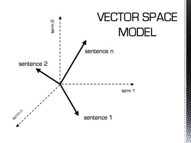
Linear Algebra Vector SpacesWhat is a Vector Space?Vector Spaces
向量空间(或线性空间)是指可以进行向量加法和数乘(称为标量乘法)的任何向量集合。
要称作向量空间 V,必须满足一系列公理。
A vector space consists of a set of vectors and a set of scalars that is closed under vector addition and scalar multiplication.
That is, when you multiply any two vectors in a vector space by scalars and add them, the resulting vector is still in the vector space.
Examples of vector spaces.
Let the scalars be the set of real numbers and let the vectors be column matrices of a specified type.
One example of a vector space is the set of all three-by-one column matrices.
If we let
对于实数元素的方阵,如果它的转置等于其逆矩阵,则被称为正交矩阵。
严格地说,矩阵 A 是正交的,如果满足 AᵀA = AAᵀ = I,其中 I 是单位矩阵。
从几何上看,一个矩阵是正交的,如果它的列向量和行向量是正交的单位向量,也就是说它们彼此垂直且大小为1。
矩阵乘法(Matrix multiplication)
矩阵乘法是线性代数中一项基础而重要的运算,用于将一个矩阵与另一个矩阵相乘,得到一个新的矩阵。
在进行矩阵乘法时,第一个矩阵的列数必须等于第二个矩阵的行数,结果矩阵的维度由这两个矩阵的行数和列数决定。
Python中计算矩阵乘法的示例:
import matplotlib.pyplot as plt
import numpy as np

# Original square defined by its corners
square = np.array([[0, 1, 1, 0, 0], [0, 0, 1, 1, 0]])

# Matrices A and B
A = np.array([[1, 2], [3, 4]])
B = np.array([[2, 0], [0, 2]])

# Apply matrix A and B transformations
transformed_square_A = np.dot(A, square)
transformed_square_B = np.dot(B, square)

# Apply matrix A then B transformation (A x B)
transformed_square_AB = np.dot(A, transformed_square_B)

# Plotting
fig, ax = plt.subplots(1, 4, figsize=(20, 5))

# Original Square
ax[0].plot(square[0], square[1], 'o-', color='grey')
ax[0].set_title('Original Square')
ax[0].set_xlim(-1, 5)
ax[0].set_ylim(-1, 5)

# Square after applying matrix A
ax[1].plot(transformed_square_A[0], transformed_square_A[1], 'o-', color='red')
ax[1].set_title('After applying A')
ax[1].set_xlim(-1, 10)
ax[1].set_ylim(-1, 10)

# Square after applying matrix B
ax[2].plot(transformed_square_B[0], transformed_square_B[1], 'o-', color='blue')
ax[2].set_title('After applying B')
ax[2].set_xlim(-1, 5)
ax[2].set_ylim(-1, 5)

# Square after applying matrix A then B
ax[3].plot(transformed_square_AB[0], transformed_square_AB[1], 'o-', color='green')
ax[3].set_title('After applying A x B')
ax[3].set_xlim(-1, 15)
ax[3].set_ylim(-1, 15)

plt.show()
迹(Trace)
矩阵的迹是其所有对角元素的和。
它在基底变换下保持不变,并提供关于矩阵的有价值的信息,即迹是矩阵特征值的和。
Python中计算迹(Trace)的示例:
# Trace of a Matrix
A = np.array([[1, 2], [3, 4]])
trace_A = np.trace(A)

print("Trace of A:", trace_A)
行列式 (Determinant)
行列式是一个与方阵的元素相关的标量值。
一个矩阵 A 的行列式通常表示为 det(A), det A 或 |A|。
其值描述了矩阵及其所代表的线性映射在给定基础下的某些特性。
特别地,当且仅当矩阵可逆且相应的线性映射是同构映射时,行列式不为零。
矩阵乘积的行列式等于各个矩阵的行列式的乘积。
2×2矩阵的行列式:
3×3矩阵的行列式:
Python中计算行列式的示例:
A = np.array([[1, 2], [3, 4]])
det_A = np.linalg.det(A)
print("Determinant of A:", round(det_A, 2))
 (Figure4:图解十进制 → 二进制)
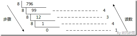
十进制 → 八进制
方法1:除8取余法,即每次将整数部分除以8,余数为该位权上的数,而商继续除以8,余数又为上一个位权上的数,这个步骤一直持续下去,直到商为0为止,最后读数时候,从最后一个余数起,一直到最前面的一个余数。
例:将十进制的(796)D转换为八进制的步骤如下:
1. 将商796除以8,商99余数为4;
2. 将商99除以8,商12余数为3;
3. 将商12除以8,商1余数为4;
4. 将商1除以8,商0余数为1;
5. 读数,因为最后一位是经过多次除以8才得到的,因此它是最高位,读数字从最后的余数向前读,1434,即(796)D=(1434)O。
(Figure4:图解十进制 → 二进制)
十进制 → 八进制
方法1:除8取余法,即每次将整数部分除以8,余数为该位权上的数,而商继续除以8,余数又为上一个位权上的数,这个步骤一直持续下去,直到商为0为止,最后读数时候,从最后一个余数起,一直到最前面的一个余数。
例:将十进制的(796)D转换为八进制的步骤如下:
1. 将商796除以8,商99余数为4;
2. 将商99除以8,商12余数为3;
3. 将商12除以8,商1余数为4;
4. 将商1除以8,商0余数为1;
5. 读数,因为最后一位是经过多次除以8才得到的,因此它是最高位,读数字从最后的余数向前读,1434,即(796)D=(1434)O。
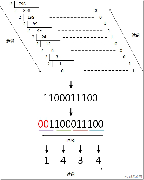
 (Figure5:图解十进制 → 八进制)
方法2:使用间接法,先将十进制转换成二进制,然后将二进制又转换成八进制;
(Figure5:图解十进制 → 八进制)
方法2:使用间接法,先将十进制转换成二进制,然后将二进制又转换成八进制;
 (Figure6:图解十进制 → 八进制)
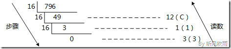
十进制 → 十六进制
方法1:除16取余法,即每次将整数部分除以16,余数为该位权上的数,而商继续除以16,余数又为上一个位权上的数,这个步骤一直持续下去,直到商为0为止,最后读数时候,从最后一个余数起,一直到最前面的一个余数。
例:将十进制的(796)D转换为十六进制的步骤如下:
1. 将商796除以16,商49余数为12,对应十六进制的C;
2. 将商49除以16,商3余数为1;
3. 将商3除以16,商0余数为3;
4. 读数,因为最后一位是经过多次除以16才得到的,因此它是最高位,读数字从最后的余数向前读,31C,即(796)D=(31C)H。
(Figure6:图解十进制 → 八进制)
十进制 → 十六进制
方法1:除16取余法,即每次将整数部分除以16,余数为该位权上的数,而商继续除以16,余数又为上一个位权上的数,这个步骤一直持续下去,直到商为0为止,最后读数时候,从最后一个余数起,一直到最前面的一个余数。
例:将十进制的(796)D转换为十六进制的步骤如下:
1. 将商796除以16,商49余数为12,对应十六进制的C;
2. 将商49除以16,商3余数为1;
3. 将商3除以16,商0余数为3;
4. 读数,因为最后一位是经过多次除以16才得到的,因此它是最高位,读数字从最后的余数向前读,31C,即(796)D=(31C)H。
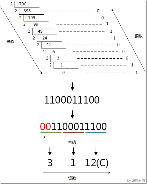
 (Figure7:图解十进制 → 十六进制)
方法2:使用间接法,先将十进制转换成二进制,然后将二进制又转换成十六进制;
(Figure7:图解十进制 → 十六进制)
方法2:使用间接法,先将十进制转换成二进制,然后将二进制又转换成十六进制;
 (Figure8:图解十进制 → 十六进制)
二进制 → 八进制
方法:
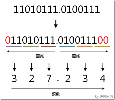
取三合一法,即从二进制的小数点为分界点,向左(向右)每三位取成一位,接着将这三位二进制按权相加,然后,按顺序进行排列,小数点的位置不变,得到的数字就是我们所求的八进制数。
如果向左(向右)取三位后,取到最高(最低)位时候,如果无法凑足三位,可以在小数点最左边(最右边),即整数的最高位(最低位)添0,凑足三位。
例:将二进制的(11010111.0100111)B转换为八进制的步骤如下:
1. 小数点前111 = 7;
2. 010 = 2;
3. 11补全为011,011 = 3;
4. 小数点后010 = 2;
5. 011 = 3;
6. 1补全为100,100 = 4;
7. 读数,读数从高位到低位,即(11010111.0100111)B=(327.234)O。
(Figure8:图解十进制 → 十六进制)
二进制 → 八进制
方法:
取三合一法,即从二进制的小数点为分界点,向左(向右)每三位取成一位,接着将这三位二进制按权相加,然后,按顺序进行排列,小数点的位置不变,得到的数字就是我们所求的八进制数。
如果向左(向右)取三位后,取到最高(最低)位时候,如果无法凑足三位,可以在小数点最左边(最右边),即整数的最高位(最低位)添0,凑足三位。
例:将二进制的(11010111.0100111)B转换为八进制的步骤如下:
1. 小数点前111 = 7;
2. 010 = 2;
3. 11补全为011,011 = 3;
4. 小数点后010 = 2;
5. 011 = 3;
6. 1补全为100,100 = 4;
7. 读数,读数从高位到低位,即(11010111.0100111)B=(327.234)O。
 (Figure10:图解二进制 → 八进制)
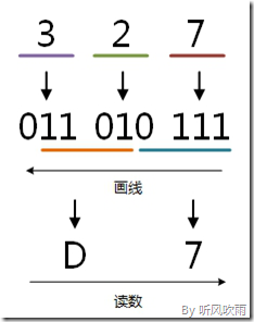
八进制 → 二进制
方法:
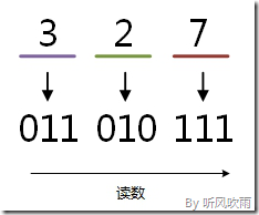
取一分三法,即将一位八进制数分解成三位二进制数,用三位二进制按权相加去凑这位八进制数,小数点位置照旧。
例:将八进制的(327)O转换为二进制的步骤如下:
1. 3 = 011;
2. 2 = 010;
3. 7 = 111;
4. 读数,读数从高位到低位,011010111,即(327)O=(11010111)B。
(Figure10:图解二进制 → 八进制)
八进制 → 二进制
方法:
取一分三法,即将一位八进制数分解成三位二进制数,用三位二进制按权相加去凑这位八进制数,小数点位置照旧。
例:将八进制的(327)O转换为二进制的步骤如下:
1. 3 = 011;
2. 2 = 010;
3. 7 = 111;
4. 读数,读数从高位到低位,011010111,即(327)O=(11010111)B。
 (Figure11:图解八进制 → 二进制)
二进制 → 十六进制
方法:
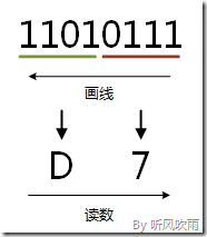
取四合一法,即从二进制的小数点为分界点,向左(向右)每四位取成一位,接着将这四位二进制按权相加,然后,按顺序进行排列,小数点的位置不变,得到的数字就是我们所求的十六进制数。
如果向左(向右)取四位后,取到最高(最低)位时候,如果无法凑足四位,可以在小数点最左边(最右边),即整数的最高位(最低位)添0,凑足四位。
例:将二进制的(11010111)B转换为十六进制的步骤如下:
1. 0111 = 7;
2. 1101 = D;
3. 读数,读数从高位到低位,即(11010111)B=(D7)H。
(Figure11:图解八进制 → 二进制)
二进制 → 十六进制
方法:
取四合一法,即从二进制的小数点为分界点,向左(向右)每四位取成一位,接着将这四位二进制按权相加,然后,按顺序进行排列,小数点的位置不变,得到的数字就是我们所求的十六进制数。
如果向左(向右)取四位后,取到最高(最低)位时候,如果无法凑足四位,可以在小数点最左边(最右边),即整数的最高位(最低位)添0,凑足四位。
例:将二进制的(11010111)B转换为十六进制的步骤如下:
1. 0111 = 7;
2. 1101 = D;
3. 读数,读数从高位到低位,即(11010111)B=(D7)H。
 (Figure12:图解二进制 → 十六进制)
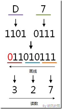
十六进制 → 二进制
方法:
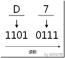
取一分四法,即将一位十六进制数分解成四位二进制数,用四位二进制按权相加去凑这位十六进制数,小数点位置照旧。
例:将十六进制的(D7)H转换为二进制的步骤如下:
1. D = 1101;
2. 7 = 0111;
3. 读数,读数从高位到低位,即(D7)H=(11010111)B。
(Figure12:图解二进制 → 十六进制)
十六进制 → 二进制
方法:
取一分四法,即将一位十六进制数分解成四位二进制数,用四位二进制按权相加去凑这位十六进制数,小数点位置照旧。
例:将十六进制的(D7)H转换为二进制的步骤如下:
1. D = 1101;
2. 7 = 0111;
3. 读数,读数从高位到低位,即(D7)H=(11010111)B。
 (Figure13:图解十六进制 → 二进制)
八进制 → 十六进制
方法:
将八进制转换为二进制,然后再将二进制转换为十六进制,小数点位置不变。
例:将八进制的(327)O转换为十六进制的步骤如下:
1. 3 = 011;
2. 2 = 010;
3. 7 = 111;
4. 0111 = 7;
5. 1101 = D;
6. 读数,读数从高位到低位,D7,即(327)O=(D7)H。
(Figure13:图解十六进制 → 二进制)
八进制 → 十六进制
方法:
将八进制转换为二进制,然后再将二进制转换为十六进制,小数点位置不变。
例:将八进制的(327)O转换为十六进制的步骤如下:
1. 3 = 011;
2. 2 = 010;
3. 7 = 111;
4. 0111 = 7;
5. 1101 = D;
6. 读数,读数从高位到低位,D7,即(327)O=(D7)H。
 (Figure15:图解八进制 → 十六进制)
十六进制 → 八进制
方法:
将十六进制转换为二进制,然后再将二进制转换为八进制,小数点位置不变。
例:将十六进制的(D7)H转换为八进制的步骤如下:
1. 7 = 0111;
2. D = 1101;
3. 0111 = 7;
4. 010 = 2;
5. 011 = 3;
6. 读数,读数从高位到低位,327,即(D7)H=(327)O。
(Figure15:图解八进制 → 十六进制)
十六进制 → 八进制
方法:
将十六进制转换为二进制,然后再将二进制转换为八进制,小数点位置不变。
例:将十六进制的(D7)H转换为八进制的步骤如下:
1. 7 = 0111;
2. D = 1101;
3. 0111 = 7;
4. 010 = 2;
5. 011 = 3;
6. 读数,读数从高位到低位,327,即(D7)H=(327)O。
 (Figure16:图解十六进制 → 八进制)
 input 3 coordinates
input pt1 x,y -> a1, a2
input pt2 x,y -> b1, b2
input pt3 x,y -> c1, c2
d = (a1 — b1) (b2 — c2) — (b1 — c1) (a2 — b2)
u = a1*a1 - b1*b1 + a2*a2 - b2*b2
v = b1*b1 - c1*c1 + b2*b2 - c2*c2
#center coordinates (x, y)
x = (u*(b2-c2) - v*(a2-b2))/d
y = (v*(a1-b1) - u*(b1-c1))/d
input 3 coordinates
input pt1 x,y -> a1, a2
input pt2 x,y -> b1, b2
input pt3 x,y -> c1, c2
d = (a1 — b1) (b2 — c2) — (b1 — c1) (a2 — b2)
u = a1*a1 - b1*b1 + a2*a2 - b2*b2
v = b1*b1 - c1*c1 + b2*b2 - c2*c2
#center coordinates (x, y)
x = (u*(b2-c2) - v*(a2-b2))/d
y = (v*(a1-b1) - u*(b1-c1))/d

 Linear Algebra Vector Spaces
What is a Vector Space?
Vector Spaces
向量空间(或线性空间)是指可以进行向量加法和数乘(称为标量乘法)的任何向量集合。
要称作向量空间 V,必须满足一系列公理。
A vector space consists of a set of vectors and a set of scalars that is closed under vector addition and scalar multiplication.
That is, when you multiply any two vectors in a vector space by scalars and add them, the resulting vector is still in the vector space.
Examples of vector spaces.
Let the scalars be the set of real numbers and let the vectors be column matrices of a specified type.
One example of a vector space is the set of all three-by-one column matrices.
If we let
Linear Algebra Vector Spaces
What is a Vector Space?
Vector Spaces
向量空间(或线性空间)是指可以进行向量加法和数乘(称为标量乘法)的任何向量集合。
要称作向量空间 V,必须满足一系列公理。
A vector space consists of a set of vectors and a set of scalars that is closed under vector addition and scalar multiplication.
That is, when you multiply any two vectors in a vector space by scalars and add them, the resulting vector is still in the vector space.
Examples of vector spaces.
Let the scalars be the set of real numbers and let the vectors be column matrices of a specified type.
One example of a vector space is the set of all three-by-one column matrices.
If we let